Excel provides an equal sign (=) as the logical operator for testing whether two expressions are the same. If you want to test whether two values differ, Excel offers another option: the not-equal-to operator. Unlike a single dedicated symbol, this operator is two characters typed as less-than followed by greater-than (<>). But if you want to use a different symbol that looks more like ≠, you’ll need to type that as Unicode.
Basic Not Equal Formula
Let’s suppose that we have two cells, A1 and B1, and we’d like to see if they’re different. We can do so using a formula such as =A1<>B1. The result of this formula is TRUE if the contents of A1 and B1 are different; FALSE otherwise.
You could also include the not-equal comparison inside a function. For instance, the IF() function has a logical-test argument, which must evaluate to either TRUE or FALSE. In this case, the formula might look like =IF(B3<>104,”Lose”,”Win”). If the value stored in cell B3 doesn’t match 104, then the function will return Lose. Otherwise, it will return Win.
Multiple Conditions with AND and OR
When evaluating multiple conditions, you can apply them explicitly using AND() or OR(). For example, the following formula tells Excel that any condition where K57900 isn’t SALES, but AJ57900 is SIC, requires review:
=IF(AND(K57900<>"SALES",AJ57900="SIC"),"Review Plan Type","")
In contrast, this one uses OR():
=IF(OR(B3<>1,C3<>0,D3<>4),"LOSE","WIN")
In both cases, the explicit comparison operators aren’t necessary; they’re simply used when you want the comparison results to be part of other calculations.
COUNTIF and SUMIF Criteria
Sometimes, the comparison needs to be made between a range and a value. For example, here’s a way to count how many numbers are in a list that don’t match a specific number:
=COUNTIF(B2:B5,”<>”&B4)
The COUNTIF() function allows us to specify criteria. Here, we’ve used quotes to indicate that we want to use the comparison symbols, and joined the not-equal operator to the value contained within cell B4.
It’s worth noting that COUNTIF() and SUMIF() operate in much the same fashion. You can use “=” and “<>” as the logical criteria in each function, provided that you enclose the expression in double quotation marks. For example, here’s a way to sum the entries in column B whose corresponding entries in column C are nonblank:
=SUMIF(C3:C6,”<>”&””,B3:B6)
Inserting the Visual Not Equal Symbol
As you know, there are times when you’d prefer the visual ≠ character to appear instead of the standard <>. To insert it, select Insert | Symbols | Symbol from the ribbon menu. Selecting Not Equal From the Symbols menu inserts the ≠ character into your worksheet. Alternatively, hold down the Alt key and type 8800 on the numeric keypad to enter the ≠ character. On a Mac, Command + Control + Spacebar opens up the Character Viewer; search for “Not Equal” to find the symbol.
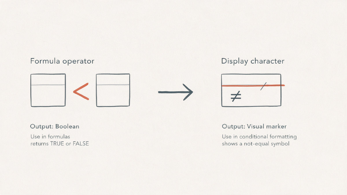
Finally, here’s our practical rule: When Excel needs to calculate the difference between values, type the < > symbols. If you just want to display the symbol for human consumption, use the ≠ character.